Feynman Diagrams

sft-wick represents Feynman diagrams as networkx.MultiGraph objects and renders them with matplotlib.

The FeynmanDiagram Class

FeynmanDiagram wraps a networkx.MultiGraph with domain-specific convenience methods.

Node types:

• External (node_type="external") — observable field operators. Rendered as filled circles.

• Vertex (node_type="vertex") — interaction vertices from \(S_{\mathrm{int}}\). Rendered as filled squares.

Edge attributes (propagators):

• kind — "C" (correlation) or "R" (response)

• index_left, index_right — component indices

• spatial_left, spatial_right — spatial arguments

Building Diagrams

Diagrams are typically constructed from a Wick pairing via the class method from_pairing():

for d_info in result.diagrams_by_order[1]:
    fd = d_info.to_feynman_diagram()

This maps each operator UID to a graph node, creates all external and vertex nodes, and adds propagator edges for each contracted pair.

You can also build diagrams manually:

from sft_wick import FeynmanDiagram

fd = FeynmanDiagram()
n1 = fd.add_external_point("phi(x)", "physical", spatial="x")
n2 = fd.add_external_point("phi(y)", "physical", spatial="y")
fd.add_propagator(n1, n2, kind="C", spatial_left="x", spatial_right="y")

Topological Properties

fd.n_loops         # E - V + connected_components
fd.is_connected    # True if the graph is connected
fd.external_nodes  # list of external node IDs
fd.vertex_nodes    # list of vertex node IDs
fd.summary()       # one-line text description

Rendering with DiagramRenderer

DiagramRenderer handles matplotlib drawing.

Single diagram:

from sft_wick import DiagramRenderer

renderer = DiagramRenderer(figsize=(8, 6))
renderer.draw(fd, title="My diagram")

Multiple diagrams in a grid:

fd_list = [d.to_feynman_diagram() for d in result.diagrams_by_order[1]]
renderer.draw_all(fd_list, ncols=3, suptitle="Order-1 Diagrams")

By default a grid has no figure-level title and uses one shared propagator legend for the whole figure. If the grid has an empty cell, the legend occupies the upper-right panel; otherwise it sits in the top figure margin. Pass suptitle=... when you want an overall title, or shared_legend=False to restore per-panel legends.

Quick Visualisation

The convenience method on PerturbativeResult handles everything in one call:

result.draw_diagrams()            # all orders
result.draw_diagrams(order=1)     # specific order

Visual Conventions

Element	Rendering
C propagator	Solid blue line
R propagator	Dashed red arrow (from \(\psi\) to \(\phi\))
External point	Filled black circle with label above
Vertex	Filled black square with coupling label below
Self-loop (tadpole)	Small circle at the node

Layout Algorithm

The renderer uses a hybrid layout:

1. networkx.spring_layout as a starting point

2. External nodes are placed on a circle (radius ext_radius, default 2.5); two-external diagrams place them mirrored on the x-axis.

3. Interaction vertices are seeded around the origin and refined by spring layout with externals pinned.

4. A post-pass enforces a minimum vertex separation (min_vertex_dist).

All four parameters are exposed via LayoutParams. When the layout result is unaesthetic for a particular topology you can pin specific nodes by passing the positions keyword to draw().

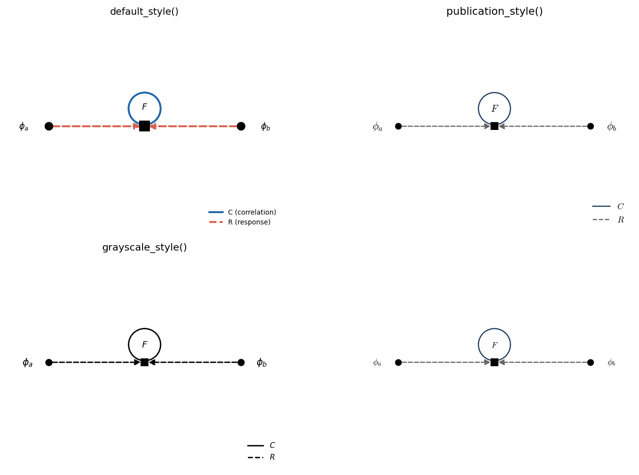
Customising the Appearance

Every visual aspect of a diagram is controlled by a RenderStyle value. Four named presets are provided:

• default_style() — the colourful on-screen look (blue C, red R).

• publication_style() — serif fonts, thinner lines, smaller markers; honours usetex.

• grayscale_style() — black-and-white for printed papers.

• minimal_style() — strips legend, boxes, and titles for inset use.

The same order-1 tadpole rendered with each preset:

from sft_wick import (
    DiagramRenderer, publication_style, LABEL_TIME_F,
)

renderer = DiagramRenderer(
    figsize=(4, 3),
    style=publication_style(),
    label_format=LABEL_TIME_F,    # \phi_a(t_f) instead of \phi_a
)
renderer.draw(fd)

Tweak a preset with with_overrides() / with_propagator():

style = (publication_style()
         .with_propagator("C", color="black", linewidth=0.9)
         .with_overrides(show_legend=False))

External-vertex labels

The label format flag controls the default text:

Flag	Default text
LABEL_COMPACT (default)	$\phi_a$ — no spatial argument
LABEL_FULL	$\phi_a(x_1)$ — pre-2026-04 default
LABEL_TIME_F	$\phi_a(t_f)$

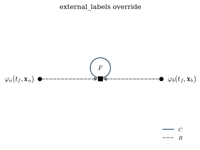
Per-call overrides win:

renderer.draw(
    fd,
    external_labels={
        fd.external_nodes[0]: r"$\varphi_a(t_f, \mathbf{x}_a)$",
        fd.external_nodes[1]: r"$\varphi_b(t_f, \mathbf{x}_b)$",
    },
)

Or supply a callable for systematic transformations:

def my_label(node_id, attrs):
    comp = attrs.get("component", "")
    return rf"$\Phi_{{{comp}}}$"

renderer = DiagramRenderer(external_label_fn=my_label)

The dictionary form in action:

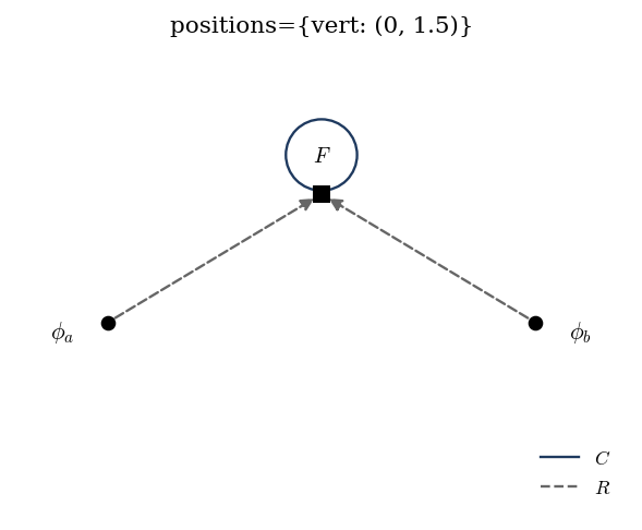
Manual node positions

When the spring layout produces something ugly for a specific topology, pin nodes explicitly:

renderer.draw(
    fd,
    positions={
        "ext_0": (-3.5, 0.0),
        "vert_2": (0.0, 1.0),
    },
)

Unpinned nodes still go through the standard layout pipeline.

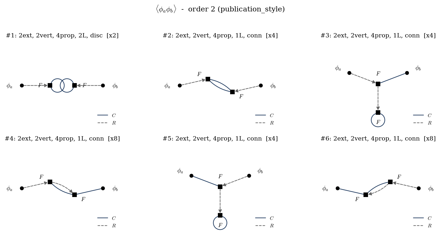
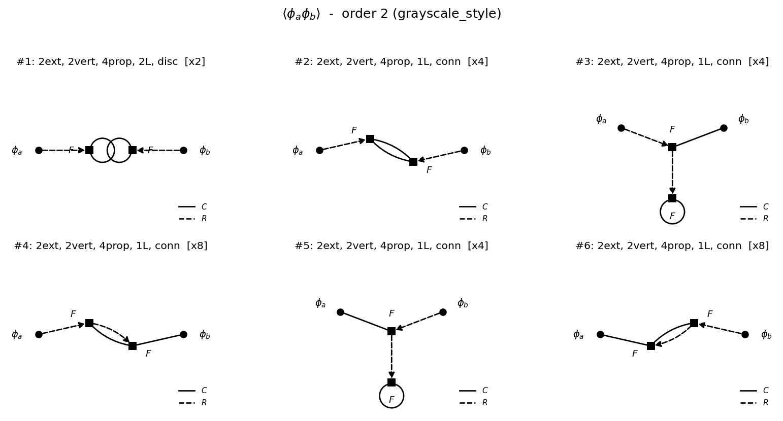
Showcase: 2-point correlator at order 2

Computing \(\langle \phi_a \phi_b \rangle_S\) to second order with a single cubic vertex

\[S_{\mathrm{int}} = F_{abc}\,\phi_a\phi_b\psi_c\]

yields six distinct topologies (with multiplicities \(2, 4, 4, 8, 4, 8\)). The grid below was produced by DiagramRenderer.draw_all() with no per-call tweaking — just publication_style():

Same diagrams in grayscale_style() for B&W reproduction:

The full reproducer is at docs/_static/diagrams/_generate.py.

Title and figure-level styling

Per-axes titles use style.title_fontsize; pass title_kwargs={…} on draw() to override that for one call. The figure-level suptitle in draw_all() honours style.suptitle_fontsize and accepts a suptitle_kwargs override. The default is no suptitle.

draw_all uses compact subplot spacing and one shared legend by default. Columns are tightened with wspace; row spacing uses a compact automatic value that is relaxed if rendered rows would overlap. Pass hspace=… to take manual control.

draw_all no longer calls plt.show() implicitly — pass show=True if you want it. This makes it safe to use inside scripts that savefig afterwards.

TikZ/PGF Backend

For LaTeX-native paper output, use TikzRenderer:

from sft_wick import TikzRenderer, publication_style

renderer = TikzRenderer(style=publication_style())

# Bare tikzpicture (drop into a paper with \input{fig.tex})
tex = renderer.to_string(fd)

# Standalone document compilable with pdflatex
renderer.save(
    fd, "fig/diag1.tex",
    standalone=True,
)

# Save many at once
diagrams = [d.to_feynman_diagram()
            for d in result.diagrams_by_order[2]]
renderer.save_all(diagrams, "fig/order2_{i:02d}.tex")

The output uses standard TikZ — your preamble needs only \usepackage{tikz} and \usetikzlibrary{arrows.meta}.

The label override hooks (external_labels, vertex_labels, external_label_fn, label_format) and positions keyword behave identically to the matplotlib backend, so you can develop the diagram interactively in a notebook with DiagramRenderer and switch to TikzRenderer for the final paper figures with no code changes beyond the class name.

A complete standalone example (compilable with pdflatex) is shipped at example.tex.